Category Archives: Algorithms

Mono.Simd and the Mandlebrot Set.

C# and .NET are some of the fastest high level languages, but still cannot truly compete with C/C++ for low level speed, and C# code can be anywhere from 20%-300% slower. This is despite the fact that the C# compiler often gets as much information about a method as the C compiler.  It has been suggested that SSE/SIMD instructions in C# could overcome some of these issues.  To evaluate this, I took a famous computational task, re-coded it using C# SIMD instructions, and evaluated the performance by looking at the execution time and how the emitted assembly code compared to the optimal assembly code.

Background

In 2009, Miguel de Icaza demonstrated a framework that allows C# to use SSE2 intrinsic operations.This is now part of the Mono library and in theory, such methods can greatly save computational time (1.5X-16X), particularly for operations on byte arrays, a common task in bioinformatics.

Test Case

Computing the mandelbrot set is one of the tasks of the computer benchmarks game, which compares program speed in different languages.  Currently, C# is listed as being slower than Java, though the programs in each language use different techniques and neither uses an optimal algorithm (see here for a better one).  However, it makes a useful test case for raw computing speed.  The challenge is to compute the picture shown below by recursively squaring a complex number and adding a constant to it.

z_{n+1} = z_n^2 + c

image_thumb[1]

The Algorithm

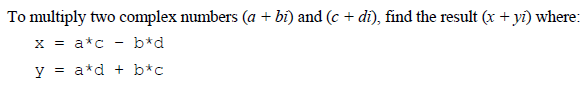
Complex numbers are a particularly challenging case because their multiplication is not a simple operation, but involves a rather annoyingly squaring of different terms and then adding/subtracting them.

image_thumb1

These are not easy vector operations, and as will be shown later one result of this is that using SSE to speed up the values for one multiplication is useless (I tried, it was worse). So, the performance improvement comes from doing two elements of the loop at a time (this is how the current Java submission is faster than the C# one, though it does not use SIMD).  The current C# version does the inner loop of the program without SIMD instructions as follows:


This loop is iterating until convergence (<4) or until the max iterations (i<0) have expired. See the wikipedia page for a full explanation.  Of interest here is that the “t” variables exist for pipelining purposes, so this is a reasonably optimized code snippet.

Trying to Implement the Optimal Solution Using Mono.Simd

Actually figuring out how to do the complex arthimetic with SSE2 is rather challenging.  Fortunately Intel published a document giving the best solution as hand coded assembly, which involves using some special SSE3 instructions I was not aware of.  Notably, the Intel optimized code is far faster than even their C code, but is only about 25% better than their optimized assembly code without SSE3.

The code below shows my attempt to implement the Intel approach in Mono.  It should be pretty fast, however it may suffer from one fatal flaw.  The comparison at the end to check for the final conditions currently requires unpacking both values in the Vector2D (when either Length.X or Length.Y have been < 4.0 at least once, then the loop stops).  The comparison for both X and Y can be done in one operation in SIMD using the built in less than statement.  However, I do not know how to turn that into a control loop function, as this requires a movmskps assembly function which mono does not seem to expose.

Results – It’s Faster on Ubuntu

img2

Shown above are the times for three different algorithms. The first is the original best submission on the website.  My SIMD submission is shown on the bottom.  Because the SIMD version does two cycles within each inner loop, as the Java submission does, I tested the Java submission converted to C# as well.  Compared to the current submission this version shows a 81% improvement, but clearly much of that is simply from doing 2 cycles in one loop.  However, even once this change is made, the SIMD instructions still give a performance boost.

The Assembly Generated is Still Not Optimal

Although the assembly generated did include lots of SSE commands, in general inspecting the assembly I noticed several things.

  1. Never unpack the double array values!  My first attempt tried to do the SSE2 steps with those instructions, and then unpack the single values as needed.  However, this failed prettty miserably, as accessing the double seemed to involve a lot of stack to register movement.

  2. All the XMM registers are not used.  The optimal version uses all of them, the C# version uses only 0-3, and soften moves things to and from the stack. Not using registers optimally seems to be a common problem though with C#.

Conclusions

The SIMD version was indeed a fair bit faster, which is nice!  However, in this case it was not a game-changer.  Most importantly though, it was really easy to use, and I think I might incorporate the byte array operations at some point in future code.  This also gave me an appreciation for assembly, which in contrast to what I had heard is easy to read and seems easy to optimize.  I just submitted the code to the shoot-out, assuming it works there it should be up soon, and I would love for someone to show me how to fix the end statement.

References   [ + ]

1. tr + ti <= 4.0) && (--i > 0

Java vs. C# Performance Comparison for Parsing VCF Files

Making a comparison with a reasonably complex program ported between the two languages.

Update 3/10/2014: After writing this post I changed the C# parser to remove an extra List<> allocation in the C# code that was not in the Java code.  After this, the Java/C# versions are indistinguishable on speed, but the C# code used ~88 MB of memory while the java version used >1GB.  Therefore, I now believe the winner is C# and a fast implementation of this parser (which can be over an order of magnitude faster for certain scenarios not in this test) is available here

VCF files are a popular way to store information about genotypic variation from next generation sequencing studies.  The files are essentially large matrices, where each element in the matrix represents a collection of information about the genotype of a particular person at a particular locus in the genome (in this sense, they can be considered as a multi-dimensional matrix in a flat file format). The Java Picard package is a common utility used for parsing these files.  While parsing, the challenge is to read each line (row) of the file, and construct objects for each element in that row that can then be manipulated or inspected.  I just finished translating the Java VCF parser in Picard to C#, and so thought it might be a good chance to compare the two different languages and runtimes. C# showed a number of advantages in the translation.  The translation itself was mostly a lot of deleting.  The get/set assessors in C# really allowed for the removal of seemingly endless amount of getXXXX/setXXX methods in Java.  It also seemed like every other line in Java was a call to some apache commons class to perform a simple task like get the maximum value in an array, create an empty list, or do a selection on data.  Extension methods and Linq have clear advantages for data processing here (though I have found these have a slight overhead relative to the for loop equivalents).  Yield statements in Java also would seem to be useful. At the same time, Java had some things that would have been nice in C#.  I had to implement basic collection types like immutable hashsets and dictionaries, a LinkedHashSet class as well as an OrderedGenericDictionary during the port.  These should be in the C# language.

Performance

This of course am what I am most interested in.  My main computer is broken, so I had to test on my windows desktop at home.  For the test, each program would read a gzipped VCF file for 20,000 lines, first creating an initial lazy class representing a portion of the data and then fully decoding this lazy version to represent the complete data as objects.  The test file was a VCF with >1,000 individuals, though unfortunately most of these individuals were non-calls at various positions, but its what I had on hand. Immediately after porting – After essentially re-writing the Java in C#, I ran some tests.  Both Java and C# can run in either client (low-memory) or server modes.  So I did both, here are the results:
Platform VM Options Working Set Paged Memory Time (s)
Java None 27.8 MB 41.32 MB 11.5
.NET None 28.9 MB 30.22 MB 15.1
Ratio 1 1.35 0.76
Java Server 362.2 MB 414 MB 7.4
.NET Server (GC) 126 MB 332 MB 14.7
Ratio 2.9 1.25 0.5
A couple noticeable conclusions here. First Java is smoking .NET on performance, but this is essentially Java code at this point and it wasn’t written for C#.  Second, there is a massive amount more memory used in server mode, and in Java at least one obtains a large performance win for this cost. After “Sharpening” the code – The initial port was basically Java, so I cleaned it up a bit after running it through the profiler, here are some notable changes:
  • String.Split winds up being a big cost in this parsing.  When porting I initially just recreated an array every time, after I realized I was recreating such large arrays I reused them as in the Java code.
  • In C# you can use unsafe pointers and I got a big performance win out of these.  I grabbed the System.String.Split code from the Mono framework, trimmed/altered it, and used it for all the split methods that seemed to be taking a long time.  The Java version also implements a custom Split method, though obviously can’t use pointers.
  • Some additional cleanup in the logic.
Platform VM Options Working Set Paged Memory Time (s)
Java None 27.8 MB 41.32 MB 11.6
.NET None 28.9 MB 30.22 MB 12.6
Ratio 1 1.35 0.92
Java Server 362.2 MB 414 MB 7.4
.NET Server (GC) 123 MB 181.61 MB 10.8
Ratio 3 2.27 0.68
So round 2, and once again Java is the winner for speed in server mode, though at a high cost in memory.  For the lower memory client model, it is nearly a tie between the two.

What explains the difference?

These programs are nearly identical but the bottleneck is not the same in both. It seems C# can split strings much faster and Java can allocate memory much faster.  Although I am less familiar with the Java profiler, it seems to show 66% of the time is spent on the String splits.  In contrast, in C# the methods that are taking up time have to do with allocating memory (constructors) and the GC, string splits are only ~17% of the total time. image image One the one hand, this means that the JVM is really doing a great job in server mode on memory allocations and other optimizations.  I can’t think why C# shouldn’t be able to match the JVM performance (perhaps dynamic recompilation is really killing it here).  On the other hand, it means that the C# program can still be improved, while I can’t really see how to improve the Java one.  The String.Split method has already been rewritten, and I didn’t see any reasonable improvements for it.  In contrast, both programs have several places where memory allocations can be saved.  For example, one aspect of the parser is that it relies on a factory class to create another class and so allocates twice the memory that it needs as it creates two large objects.  Simply having one object be it’s own factory would solve this.  Similarly, several empty lists are repeatedly created that could point to the same list or simply be skipped.  I wanted this parser to generally match the Java version, so did not pursue these changes, but my guess is they may shrink the difference (though again, in Java this clearly didn’t matter).

Conclusions

The JVM is the clear winner on speed, particularly in server mode where memory isn’t an issue.  C# was the clear winner on brevity, syntax and language features.  The difference was only substantial in server mode, and the C# program (and likely the Java program) were far from optimal, but it gives a rough hint at how they compare.  The next question will be how they compare when C# runs with mono on a Linux environment.

Not All Poisson Random Variables Are Created Equally

Spurred by a slow running program, I spent an afternoon researching what algorithms are available for generating Poisson random variables and figuring out which methods are used by R, Matlab, NumPy, the GNU Science Libraray and various other available packages. I learned some things that I think would be useful to have on the internet somewhere, so I thought it would be good material for a first blog post. Many meaningfully different algorithms exists to simulate from a Poisson distribution and commonly used code libraries and programs have not settled on the same method. I found some of the available tools use inefficient methods, though figuring out which method a package used often required me to  work through the source code.
(from Wikipedia)

(from Wikipedia)

This blog post explains the specific algorithms that commonly used packages implement. For those looking for the quick take away, the lesson is to avoid the default Matlab implementation and the GNU Science Library (GSL). For context, when deciding which Poisson simulation routine to use there are essentially two important questions. The first is if you will be repeatedly simulating values conditioned on the same mean parameter value (λ).  If so, methods that that store certain pre-computed information offer very big performance improvements.  However, essentially no package implements these routines (with some exceptions discussed at the end).  The second question is if you are frequently going to simulate with a λ > 10.  Poisson simulation methods usually switch between two different methods depending on if λ is above or below 10 (this “decision value” can change slightly but seems to always be >=10).  When λ is below 10, the algorithms are all very similar and their speed scales with the value of λ.  Where the algorithms really differ is how fast they are when  λ > 10. For λ > 10, the GNU Science Library (GSL) and Matlab have slower algorithms that are of order log(λ).  Their methods are straightforward implementations from pages 137-138 of Knuth’s Seminumerical Algorithms book  (specifically the 1998 version, older versions had a more inaccurate algorithm). On these pages Knuth’s book presents a 1974 algorithm by Aherns and Dieter [1] but he unfortunately only introduces the more efficient algorithm from Aherns and Dieters’ 1982 paper [2] with an excercise buried at the end of the chapter.  This was an understandable decision given the complexity of the 1982 method, but it is somewhat unfortunate for Matlab and GSL users. A major breakthrough in algorithms for Poisson random generators came with the publication of the first O(1) algorithm in 1979 by Atkinson [3] and methods from then on are signifcantly better. The Math.NET  project uses this 1979 algorithm in their sampler.  A still better method is the 1982 Aherns and Dieter method which is also heavily used.  For example, the R Project  uses this efficient algorithm.  Importantly, the R version also checks to see if it can avoid recomputing values if the same λ value is being used on repeated function calls. To me, this is just another example of how great the core R implementations often are.  Although in my field the GSL seems to dominate when people code, I think a reason for this is that a lot of people don’t realize that many R functions can be easily incorporated into C/C++ code using the R Stand Alone Math Library.  I have found simulating with the R libraries has many advantages over using the GSL. In 1986 Luc Devroye published a real tome on Random Variate Generation (that is freely available online).  Within it was a very good algorithm, which I gather is based on a 1981 paper, that is currently implemented by the Infer .NET package and the Apache Commons Math Java library.  The algorithm is given on page 511 of the book, but anyone independently implementing it should be aware that the published errata corrects some errors in the original publication of this algorithm (Infer.NET has these corrections, but I didn’t check for them in the Apache Commons library). The most modern algorithm I found implemented was a 1993 algorithm by Hormann [5], which his benchmarks showed either outperformed other algorithms at many λ values, or was not that meaningfully slower over a narrower range of λ values. Numpy implements this routine, and it seems at least one commentator on another blog  implemented it as well. So which to use?  I think one should make sure they are using a post-1979 algorithm (so not Matlab or GSL).  Routines after this point are similar enough that if simulating Poisson variables is still the bottleneck one should benchmark available code that implements these different options.  At this point the coding/implementation specifics, and the ease of using that library, will likely be more important than the algorithm.  If no available option adequately performs, the algorithms in [2], [4] and [5] can be evaluated for application to a specific usage scenario, though by then it is probably worth knowing that the algorithms that are truly the fastest have efficient pre-computed tables or a particular λ  value [6] .  One such table lookup method from reference [6] is implemented in Matlab code available from an open source file exchange here.  Though I did not completely evaluate [6], the 2004 paper says it can outperform (5X-15X faster) the other algorithms I have discussed.  However, after a quick run through of the paper, I couldn’t tell if the benchmarks in [6] were based on repeated simulations from the same λ value, or with constantly changing λ values (I suspect it is the former which is why this algorithm is not widely adopted).  The algorithm in [6] strikes me as very efficient for the same λ value, and C code for it is available from the publishing journal.  Interestingly, a Matlab benchmark test shows this method is about 10X faster than the default poissrnd Matlab function, even though it recreates the required look up tables on each function call.  However, I suspect the performance increase is slightly exaggerated because the original Matlab function has such a slow routine and this method switches directly to the normal approximation of the Poisson distribution when λ is over 1,000.  This shortcut could easily be incorporated to every other method mentioned, though the direct methods seem fast enough that I personally would not like to muck around evaluating how well one distribution mathematically approximates another distribution that itself is only approximating a complex reality. Which brings me to the end of the first blog post.  If you are still reading this you slogged through some insights gained from someone who just read Fortran code and academic papers from a time when Nirvana was still just a Buddhist goal and not a grunge rock band.  Hopefully it prevents someone else from doing the same.

    References

1. Ahrens JH, Dieter U (1974) Computer methods for sampling from gamma, beta, poisson and bionomial distributions. Computing 12: 223-246. 2. Ahrens JH, Dieter U (1982) Computer generation of Poisson deviates from modified normal distributions. ACM Transactions on Mathematical Software (TOMS) 8: 163-179. 3. Atkinson A (1979) The computer generation of Poisson random variables. Applied Statistics: 29-35. 4. Devroye L (1986) Non-uniform random variate generation: Springer-Verlag New York. 5. Hörmann W (1993) The transformed rejection method for generating Poisson random variables. Insurance: Mathematics and Economics 12: 39-45. 6. Marsaglia G, Tsang WW, Wang J (2004) Fast generation of discrete random variables. Journal of Statistical Software 11: 1-11.